An easy way to think about mathematical expressions-calculation graph
Editor's note: Backpropagation is a common method for training artificial neural networks. It can simplify the computational processing of deep models. It is a key algorithm that beginners must master. For modern neural networks, through backpropagation, we can greatly increase the training speed of the model with gradient descent, and complete the model that may have taken 20,000 years for researchers to complete in one week.
In addition to deep learning, the backpropagation algorithm is also a powerful calculation tool in many other fields, from weather forecasting to analyzing numerical stability-the only difference is the name difference. In fact, this algorithm has mature applications in dozens of different fields, and countless researchers are fascinated by this form of "reverse mode derivation".
Fundamentally speaking, whether it is deep learning or other numerical computing environments, this is a convenient and fast calculation method, and it is also an essential calculation trick.
Calculation graph
When it comes to calculations, some people may have a headache for annoying calculation formulas, so this article uses an easy way to think about mathematical expressions-calculation graphs. Take the very simple e=(a+b)×(b+1) as an example. From a computational point of view, it has a total of 3 operations: two summation and one product. In order for everyone to have a clearer understanding of the calculation graph, here we calculate it separately and draw the image.
We can divide this equation into 3 functions:

In the calculation graph, we put each function together with the input variables into the node. If the current node is the input of another node, use a cut-out line to indicate the data flow direction:
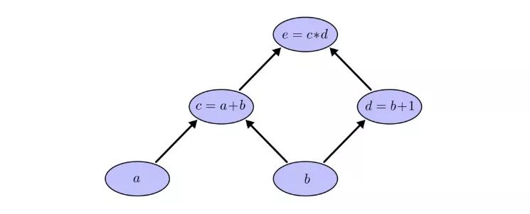
This is actually a common description method in computer science, and it is very useful especially when discussing programs involving functions. In addition, most of the popular deep learning open source frameworks, such as TensorFlow, Caffe, CNTK, Theano, etc., all use computational graphs.
Still taking the previous example as an example, in the calculation graph, we can calculate the expression by setting the input variable to a specific value. For example, we set a=2 and b=1:
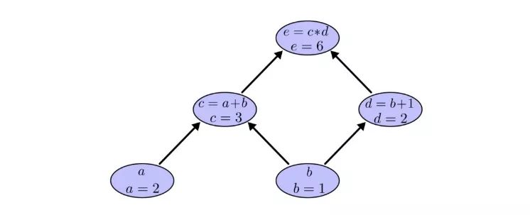
We can get e=(a+b)×(b+1)=6.
Calculate the derivative on the graph
If we want to understand the derivative on the calculation graph, a key is how we understand the derivative on each arrowed line (hereinafter referred to as "side"). Take the previous edge connecting node a and node c=a+b as an example. If a has an effect on c, what kind of effect is this? If a changes, how will c change? We call this the partial derivative of c with respect to a.
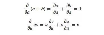
In order to calculate the partial derivatives in the graph, let's review these two summation rules and product rules first:
Given that a=2 and b=1, the corresponding calculation diagram is:
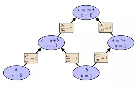
Now we have calculated the partial derivatives of two adjacent nodes. If I want to know how the nodes that are not directly connected affect each other, what would you do? If we input a with a speed change of 1, then according to the partial derivative, the rate of change of the function c is also 1. It is known that the partial derivative of e relative to c is 2, then the same, the rate of change of e relative to a is also 2. .
The general rule for calculating the partial derivative between nodes that are not directly connected is to calculate the sum of the partial derivatives of each path, and the partial derivative of the same path is the product of the partial derivatives of each side. For example, the partial derivative of e with respect to b is equal to:
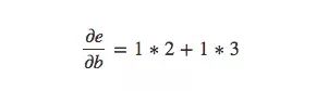
The above formula shows how b affects function e by influencing functions c and d.
Such a general "path sum" rule is just a different way of thinking about the multiple chain rule.
Path decomposition
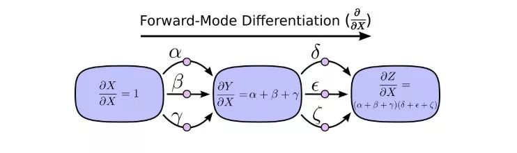
The problem with "path summation" is that if we simply and crudely calculate the partial derivative of each possible path, we are likely to end up with an "explosive" sum.
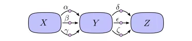
As shown in the figure above, there are 3 paths from X to Y, and 3 paths from Y to Z. If we want to calculate ∂Z/∂X, we need to calculate the sum of the partial derivatives of 3×3=9 paths:
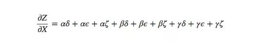
This is only 9 items. As the model becomes more and more complex, the corresponding computational complexity will also increase exponentially. Therefore, rather than silly summing up one by one, we'd better remember some elementary school mathematics and then convert the above formula to:

Is it familiar? This is the most basic partial derivative equation in the forward propagation algorithm and the back propagation algorithm. By decomposing the path, this formula can calculate the sum more efficiently. Although there is a certain difference between the length and the sum equation, it is indeed only calculated once for each edge.
The forward mode derivation starts from the input of the calculation graph and ends at the end. At each node, it summarizes all the input paths, and each path represents a way the input affects the node. After the addition, we can get the total impact of the input on the final result, which is the partial derivative.
Although you may not have thought of understanding from the perspective of computational graphs before, when you look at it this way, in fact, the forward mode derivation is similar to what we were exposed to when we first started learning calculus.
On the other hand, the reverse mode derivation starts from the end of the calculation graph to the end of the input. For each node, what it does is merge all paths that originate from that node.

The forward mode derivation focuses on how an input affects each node, and the backward mode derivation focuses on how each node affects the last output. In other words, the derivation of the forward mode is filling ∂/∂X into each node, and the derivation of the backward mode is filling ∂Z/∂ into each node.
You're done
Speaking of now, you might be wondering what the meaning of reverse mode derivation is. It looks like a strange version of the derivation of the forward model. Is there any advantage in it?
Let's start with the previous calculation diagram:

We first use the forward mode to calculate the influence of input b on each node:
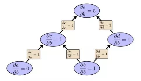
∂e/∂b=5. Let's put this aside, let's take a look at the reverse mode derivation:
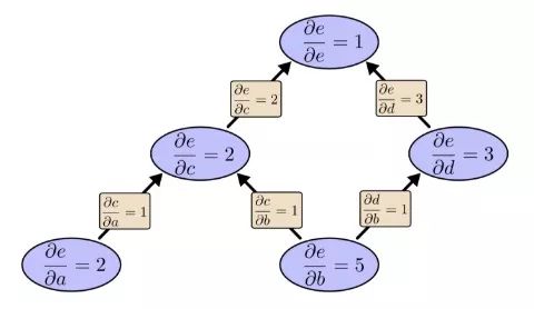
Earlier we said that the reverse mode derivation focuses on how each node affects the final output. According to the above figure, we can find that the partial derivatives in the graph have both ∂e/∂b and ∂e/∂a. This is because this model has two inputs, and both of them affect the output e. In other words, the reverse mode derivation can better reflect the global input situation.
If this is a simple example with only two inputs, and neither method does matter, then imagine a model with one million inputs and only one output. For a model like this, we need to calculate the derivation in the forward mode a million times, and the derivation in the reverse mode only needs to be calculated once. This is a good judgment!
When training a neural network, we regard cost (a value describing how well the network performs) as a function containing various parameters (numbers describing how the network behaves). In order to improve the performance of the model, we have to continuously change the parameters to derive the cost function to perform gradient descent. The model has tens of millions of parameters, but its output is only one, so machine learning is a suitable application field for the reverse mode derivation, that is, the back propagation algorithm.
Is there a case in which the forward mode derivation is better than the reverse mode derivation? some! What we have talked about up to now is the multi-input single-output situation. In this case, the reverse is better; if it is one-input multiple-output, multiple-input multiple-output, the forward mode is faster to derive!
Isn't this too common?
When I really understood the backpropagation algorithm for the first time, my reaction was: Oh, the simplest chain rule! Why did it take me so long to understand? In fact, I am not the only one who has this kind of reaction. Indeed, if the problem is that you can derive the smarter calculation method from the derivation of the forward mode, it will not be so troublesome.
But I think this is more difficult than it seems. When the backpropagation algorithm was first invented, people actually did not pay much attention to the research of feedforward neural networks. So no one found that its derivatives are conducive to fast calculations. But when everyone knew the benefits of such derivatives, they began to react again: it turns out that they have such a relationship! There is a vicious circle in this.
To make matters worse, it is very common to push algorithm derivatives in your head. When it comes to training neural networks with them, it is almost equivalent to a scourge. You will definitely fall into a local minimum! You may waste huge calculation costs! People will shut up and practice only after confirming that this method is effective.
summary
Derivatives are easier to explore and better to use than you think. I hope this is the main experience this article brings you. Although in fact this mining process is not easy, it is important to understand this in deep learning. From another perspective, we can discover different landscapes. The same applies to other fields.
Any other experience? I think there is.
The backpropagation algorithm is also a useful "shot" to understand the process of data flowing through the model. We can use it to know why some models are difficult to optimize, such as the problem of the disappearance of gradients in the classic recurrent neural network.
Finally, readers can try to combine forward propagation and back propagation algorithms for more effective calculations. If you really understand the techniques of these two algorithms, you will find a lot of interesting derivative expressions.
Some client may feel that 10th Laptop is little old, so prefer 11th Laptop or 12th laptop. However, you will the 10th cpu is even more powerful than 11th, but price is nearly no difference, especially you take in lot, like 1000pcs. As a professional manufacturing store, you can see Laptop i3 10th generation 8gb ram,i5 laptop 10th generation, intel i7 10th gen laptop, etc. It`s a really tough job selecting a right one on the too many choices. Here are some tips, hope help you do that easier. Firstly, ask yourself what jobs you mainly need this Gaming Laptop to do. Secondly, what special features you care more? Like fingerprint, backlight keyboard, webcam rj45, bigger battery, large screen, video graphics, etc. Finally, ask the budget you plan to buy gaming laptop. Thus you will get the idea which laptop is right one for you.
Except integrated laptop, also have graphic laptop with 2gb or 4gb video graphic, so you can feel freely to contact us anytime and share your basic requirements, like size, cpu, ram, rom, video graphics, quantity,etc. More detailed value information provided in 1-2 working days for you.
10th Laptop,Laptop I3 10th Generation 8gb Ram,I5 Laptop 10th Generation,10th Generation Laptop,Intel I7 10th Gen Laptop
Henan Shuyi Electronics Co., Ltd. , https://www.shuyitablet.com